![]()
![]()
![]()
3.Damping effect
We have explained how to determine damping ratio and loss factor on the assumption that the amplitude attenuates exponentially so far. Now we will briefly explain what damping ratio physically means in vibration.
3-1 Damping effect in free vibration
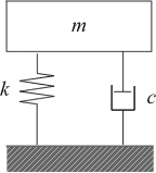
Free vibration is vibration which no external force is applied to. If no external force is applied, it will remain to stand still. However, if an initial displacement or initial velocity is added as initial condition, the vibration will start. Taking the spring mass model shown in Fig. 4 as an example, first pull the mass m of block, add a displacement (initial displacement) onto the spring k and release it suddenly, then the vibration start. This is the free vibration.
Fig.4 Free vibration model |
If the damping force c is zero, the free vibration will permanently continue. The vibration frequency ω0 is expressed in the following equation.
 |
(11) |
ω0 is called as natural frequency. From experience, free vibration does not last indefinitely. The damping force c works, the amplitude gradually decreases as illustrated in Fig. 1 and eventually it will stop. The behavior differs depending on whether the value of c is larger or smaller than ccin the following equation.
(12) |
cc is called as critical damping coefficient, the ratio of cc and c is the subject of this article,
ζ (damping ratio).
(13) |
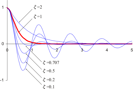
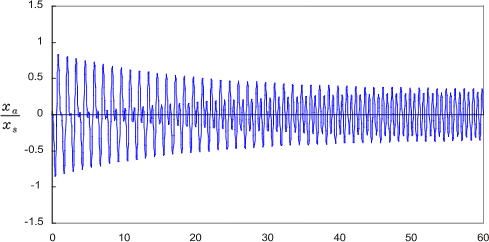
As mentioned above, the amplitude or free vibration changes according to ζ (damping ratio). The example is shown in Figure 5.
Fig.5 Response of free vibration |
If ζ < 1, the amplitude of damped free vibration is shown in the following equation.
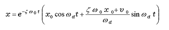 |
(14) |
x0: initial displacement
v0: initial velocity
ωd is called as natural frequency of vibration system and shown in the following equation.
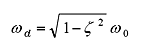 |
(15) |
ωd is somewhat smaller than ω0. Actually ωd is close to ω0 as the value of ζ is small in the actual vibration system. As seen in Equation (14), the behavior of the damped vibration system is determined by the initial conditions and the damping ratio ζ. If the initial velocity as 0, initial displacement as 1, the response due to difference in damping ratio ζ is shown in Figure 5. It can be seen that the behavior varies greatly depending on the damping ratio ζ.
If ζ ≥ 1, it cannot be calculated by equation (14), but by another equation. For comparison, those responses are shown in Figure 5. ζ =1 is called as critical damping, ζ >1 as over damping, 1>ζ >0 as underdamping. In Fig. 5, ζ = 1 (critical damping) is emphasized for ease of understanding, but this only indicates the boundary of whether or not it vibrates, and it does not mean that critical damping is particularly important.
The response is shown in Fig.5 if ζ =0.707 (=![]() ), this is important for steady-state vibration. Although there is some overshoot (undershoot), it is a value that is often used when the response time is important for control system, as the value that minimizes the settling time (which is the response to converge within 5% of the target value).
), this is important for steady-state vibration. Although there is some overshoot (undershoot), it is a value that is often used when the response time is important for control system, as the value that minimizes the settling time (which is the response to converge within 5% of the target value).
3-2 Damping effect in steady-state vibration
Next, we explain about the case where a continuous force is applied to the free vibration system from the outside.
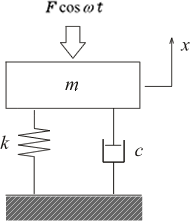
When external force is applied, it is called forced vibration. When the external force is a sine wave and sufficient time has passed (steady-state), it is called steady-state vibration. While, the state before steady-state is called a transient state, it will be explained later.
As shown in Figure 6, we look into a model in which exciting force ![]() is applied to single-degree-of-freedom vibration system. Symbols and equations are shown as follow:
is applied to single-degree-of-freedom vibration system. Symbols and equations are shown as follow:
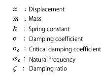 |
Fig.6 Model of exciting forced vibration |
|
(11) |
| (12) | |
| (13) |
Since the exciting force is a repetitive force of frequency ω, steady-state vibration driven by the exciting force will also be the same frequency. However, amplitude and phase are different. Thus, we obtain them as below.
The equation of motion of the system shown in Fig. 6 is expressed by the following equation. By solving this equation, amplitude and phase of steady-state vibration can be obtained.
(16) |
Equation of steady-state vibration is;
(17) |
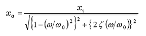
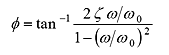
Amplitude xa and phase φ are shown as follow
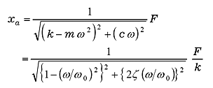 |
(18) |
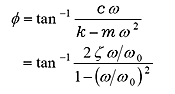 |
(19) |
In Equation (18), F / k is the static displacement when static force F is applied. To replace F / k with xs, equation (18) is
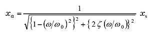 |
(20) |
In other words, the amplitude of steady-state vibration is expressed as a frequency response functionality of static displacement xs, natural frequency ω0, and damping ratio ζ .
Equation (20) is changed to;
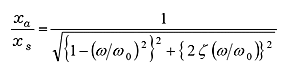 |
(21) |
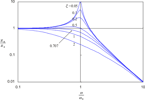
is called amplitude magnification. Fig 7 is shown in the logarithm, taking ω / ω0 on the horizontal axis and amplitude magnification on the vertical axis. This figure finds steady-state vibration is resonated around ω0, and amplitude magnification is greatly affected by damping rate ζ.
Fig.7 Amplitude magnification |
The characteristic of amplitude magnification is summarized here:
When ![]() , it has one resonance point at
, it has one resonance point at ![]() as resonance frequency. Bigger ζ is, smaller resonance frequency ωr is. When ζ is small (around ζ <0.05), it resonates with natural vibration but it doesn’t resonate with
as resonance frequency. Bigger ζ is, smaller resonance frequency ωr is. When ζ is small (around ζ <0.05), it resonates with natural vibration but it doesn’t resonate with ![]() .
.
Amplitude magnification is maximum at resonance frequency.
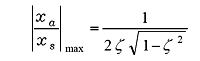 |
(22) |
When ζ is small;
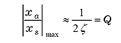 |
(23) |
It is equal to Q. It means that it is often treated as Q when resonance is sharp.
Amplitude magnification is close to 1 at frequency lower than resonance point.
Amplitude magnification is close to![]() , that is slope of -40 dB/decade.
, that is slope of -40 dB/decade.
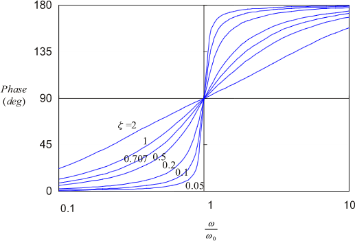
Phase difference between exciting force and steady-state vibration is shown in equation (19). This is shown graphically in Fig.8.
Fig.8 Phase lag of steady-state vibration |
When frequency of exciting force is lower than ω0 (lower frequency range), phase lag of steady-state vibration is close to 0 deg, that is steady-state vibration is vibrated at phase slightly delayed from exciting force.
In frequency range higher than ω0, phase lag of steady-state vibration is close to 180 deg, that is steady-state vibration is vibrated at opposite phase from exciting force.ζ is small, phase is drastically changed, while ζ is bigger, the change is gentle.
3-3 Damping effect in transient vibration
In the previous article, we explain about steady-state vibration when enough time has passed since the external force was applied. Now we explain about transient state, which is the state from the external force is applied until reading steady-state.
Considering the vibration system in Fig. 6, the equation of motion is Equation (24), however, for easy to understand, we assume external force is ![]() and the initial condition is completely stationary, that is, the initial displacement and initial velocity are zero.
and the initial condition is completely stationary, that is, the initial displacement and initial velocity are zero.
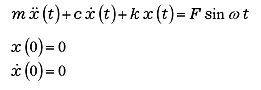 |
(24) |
As this system is linear, principle of superposition is true. The solution is obtained in the form of the sum of the vibration components by external force and the free vibration component.
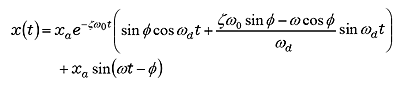 |
(25) |
 |
(26) |
 |
(27) |
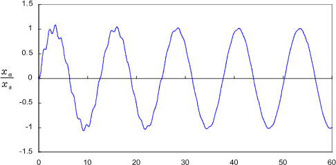
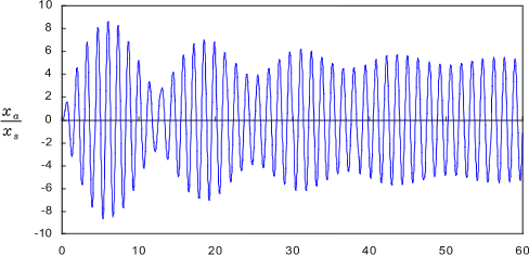
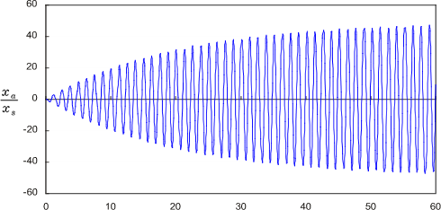
The first term of equation (25) is a free vibration component, it is attenuating gradually, and finally only the steady-state vibration component of the second term remains. This is shown in Figure 9-1 to 9-4. Here is ζ = 0.01, the change in the transient response is shown when ω/ω0 is changed to 0. 1, 0. 9, 1. 0, and 2. 0.
When ω/ω0 is small, the free vibration is gradually attenuated over time and become steady-state vibration as free vibration superimposed steady-state vibration.
When ω/ω0 is close to 1, that is when the excitation frequency approaches the natural vibration frequency, the amplitude increases and the beat is generated.
When ω/ω0 = 1, that is the excitation frequency is equal to natural frequency, the amplitude increases in proportion to time, and become resonance state.
When ω/ω0 >1, the amplitude is reducing but become complicated waveform.
Here, ζ = 0. 01 is set to small value to make the transient state easy to understand. However, if ζ is large, the free vibration converges quickly and the amplitude of steady-state vibration also decreases. That amplitude is shown as in Fig.7. On the other hand, if ζ is small, the transient state does not converge soon, and the unstable state will continue for a long time. In particular, at frequencies near ω/ω0 = 1, even with a small vibration at first, the amplitude gradually increases and become very large vibration. (Note; the scale of vertical axis is different in Fig.9-1 to 9.4)
| Fig. 9-1
ζ =
0.01 |
|
| Fig. 9-2
ζ =
0.01
|
|
| Fig. 9-3
ζ =
0.01
|
|
| Fig. 9-4
ζ =
0.01
|
|