16.Necessity of FFT zooming analysis
The following graph represents that five types of materials with different loss factors were measured with different frequency resolutions when performing FFT zooming analysis. The horizontal axis shows the number of FFT measurement points within -3 dB as in half valued method. As the zoom magnification is increased as shown below, the measured η gradually converges to the constant value.
Using this value as true, the errors are calculated as shown in the rewritten graph.
|
|
If the resolution point of the FFT within half value width is approximately 15 points, the measurement accuracy of the loss factor will be about 1%. In case loss factor is small, the zoom analysis is necessary.
17.Zoom analysis and Mass cancelation
The figure below shows the measurement errors of loss factor are caused by performing or not performing zoom analysis and mass cancelation. By performing both zoom analysis and mass cancellation, the errors are most minimized. Please take note that the difference of loss factor caused by performing or not performing zoom analysis and mass cancelation is remarkably seen in case of loss factor as 0.01 or less.
|
Performing zoom analysis or not greatly affect the loss factor than performing mass cancellation.
18.Curve fitting by use of pole-zero models for the loss-factor measurement
(At present, it is considered to be the best curve fitting method for loss factor measurement, so we’ve obtained the approval of Prof. Hideo Suzuki of Chiba Institute of Technology to publish the paper as it is.)
1.Introduction
With the recent progress in manufacturing engineering of damping materials, we are making practical usage of materials with large loss factors. There is only a traditional half-width method for the standardized measurement method of loss factor including ISO. Here, the half-width method is a method defined by η =(f2- f1)/ f0 which is calculated by the resonance frequency
f0 obtained from the vibration response characteristics such as amplitude, velocity, acceleration, and the frequencies f1 and f2 at which the response decreases by 3 dB from the resonance peak level. However, the materials with a difference in level between resonance and anti-resonance of less than 3 dB have been developed recently, the half-width method is not useful at all for such materials. Furthermore, as a recent Engineering trend, an attempt is made to obtain a loss factor from the sharpness of the resonance frequency characteristics and the sharpness of the anti-resonance characteristics. For example, instead of using the peak (the resonance characteristics) of the frequency response functions obtained from [Velocity/force], the loss factor is obtained from the bottom one (the anti-resonance characteristics). Although the relationship between the sharpness of anti-resonance and the value of the loss factor at that frequency is not clear, it is necessary to fit the both characteristics of resonance and anti-resonance in case using the materials with not a little of differences between the peak and the bottom.
For the above mentioned reason, It is recommended to employ the pole-zero models in which the loss-factor is measured by curve fitting to the characteristics of [velocity/force] or [force/velocity]. This paper will explain the overview.
2.The Pole-zero models
The Pole-zero model is a characteristic that expresses the response characteristic at the excitation point as following:
|
or
|
ηn represents the dullness of the characteristics at each resonance and anti-resonance (in case of resonance, it is loss factor). Ωn represents resonance or anti-resonance, H represents constant. (1) and (2) represent ether impedance ([force/velocity]) or mobility ([velocity/ force]), here’s mobility.
The mobility of cantilever corresponds to (2), the mobility of free-free beam corresponds to (1) as each mobility increases or decreases according to the frequency approaches zero. When fitting to the impedance characteristic, the inverse may be taken, and therefore, the equations may be replaced and applied. The greatest characteristics of the pole-zero model is that the loss factor (also called the loss factor for convenience in the case of anti-resonance) is shown as explicit, it means the sharpness of peak and bottom characteristics is independent]y defined. For your reference, the calculation used for mode analysis is shown as below. The loss factor at resonance can only be input as explicit.
|
3. Error function for the curve fitting
Error function that expresses the differences between actual data and model characteristics is necessary to be devised to fit the same error to peak and bottom of characteristics. It is common use for error function as follow:
|
A(Ω m)is actual characteristics, X(Ω m)is model characteristics. Since the number is great in resonance, even the same % of error contributes greatly, and the characteristic error in anti-resonance is neglected. There are 2 error functions introduced to solve this problem.
|
Formula (5) is a method that uses characteristic expressing frequency response functionality in decibels for fitting. Formula (6) is a method that the same error rate in the peak and bottom contributes to λ with the same magnitude by normalizing with the measured characteristics. By using these error functions can make it possible to simultaneously fit the resonance and anti-resonance characteristics.
4.Application for model data
It is available to calculate the characteristics from Formula (1) or (2), regard it as actual measurement data, perform fitting, check how close to the true value can be obtained, and verify the correctness of the algorithm. Fig. 1 shows the result. The thin solid line with four poles and zeros has the characteristic to be fitted and is calculated by giving the loss factor corresponding to the resonance and anti-resonance frequencies of the type B pole-zero model in Fig. 1. The resonance and anti-resonance frequencies correspond to the frequency distribution during the central exciting with rectangular beam. The loss factor 0.1, 0.2 and 0.3 are appropriately allocated to each resonance and anti-resonance. The thick line is calculated by the loss factor uniformly given to an initial value of 0.15. and having random positive or negative 10% errors to the resonance and the anti resonance frequencies.
It is calculated by giving decibel type error functionality. After fitting using the decibel type error functionality, the correct parameter value is obtained with an accuracy of 8 digits or more. (The converged curve overlaps the thin line.) The advantage of obtaining the loss factor by curve fitting is that the frequency resolution may be much rough than the half-width method when measuring. The fitting is available, even if it is rough enough to look like a line graph at low frequencies as shown Fig1.
|
5.Actual measurement with the curve fitting method
Correspondence to the small loss factor
The measurement errors for the loss factor overlay the graph which represents number of measurement points within half value width as following figure. It can be seen that if there is a measuring point of about 0.3 point within the half value width, the errors are within a few percent.
|
black line: half value width method ±(1/m2+1/m)line
red line: half value width method ±(1/m2)line
purple line: curve fitting method necessary line
Correspondence to the big loss factor
The frequency response functionality that cannot be measured by the half value width method under simulationη= 0.7,1.0,1.2 is performed by curve fitting with dB method as shown below. It enables to measure with high accuracy up to the 6th resonance frequency at around 0.7 loss factor, up to 3rd resonance frequency at around 1.0, 1.2 loss factor.
|
19.Two points hanging method
This is a method of hanging a node for each vibration mode. As it can be measured from the smallest loss factor by hanging at a position where does not move, it is mainly used for the measurement of loss factor for single metal product. The disadvantage of this method is that the hanging position must be changed for each mode. It is common to use non contactable electromagnetic excitation for excitation and use it as electromagnetic velocity sensor for response. (As for the electromagnetic excitation/detector, please refer to the devices for cantilever method.
|
Position of
| degree | 1 | 2 | 3 | 4 | 5 |
|---|---|---|---|---|---|
Position of node |
22.42 | 13.21 | 9.44 | 7.35 | 6.01 |
| 50.00 | 35.58 | 27.68 | 22.65 | ||
| 86.79 | 64.42 | 50.00 | 40.91 | ||
| 90.56 | 72.32 | 59.09 | |||
| 92.65 | 77.35 | ||||
| 93.99 |
*The position from the left and right ends is expressed in % when the length of the test beam is 100%. If there are many nodes, you may hang anywhere.
20.The loss factor depends on the vibration mode
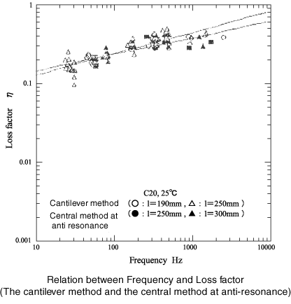
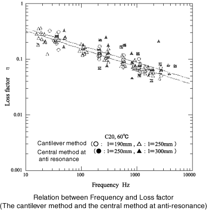
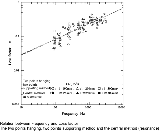
According to the relation between testing method and the vibration mode as below, the vibration mode by the cantilever method and the central excitation method is same when the length of specimen beam for the cantilever method is a half of the length of specimen beam for the central exciting method. The vibration mode by two points hanging, two points supporting method at resonance and the central exciting method at resonance is same.
|
The following 4 figures show the comparison of loss factor for 1. the cantilever method at resonance and the central exciting method at anti-resonance, and 2. the two points hanging, two points supporting method at resonance and the central exciting method at anti-resonance. These figures find it as follow:
The cantilever method≠the central exciting method(at anti-resonance)
The two points hanging, two points supporting method≠ the central exciting method (resonance)
The valid length of specimen beam
2 times of cantilever method = the central exciting method


