No.14 Displaying time waveform of velocity/displacement
Three physical quantities are generally used to quantitatively capture vibrations: displacement (m), velocity (m/s), and acceleration (m/s2). There are various types of sensors for measuring vibration, and they are classified into displacement, velocity, and acceleration sensors according to the physical quantity.
Piezoelectric accelerometers are contact-type and relatively easy to handle, but can only measure acceleration. When measuring velocity or displacement, the signals obtained from the accelerometer are converted to velocity or displacement by numerical integration.
If the acceleration time waveform is just converted by numerical integration, the correct velocity or displacement waveform is not obtained due to low frequency noise. In such a case, IFFT (inverse-Fourier transform) function is used. In this column, I will introduce how the time waveform of velocity or displacement is displayed by taking the DS-0321 FFT Analysis function.
Time waveform and spectrum for vibration acceleration of pendulum
The figure 1 shows the time waveform and power spectrum of the vibration acceleration when the accelerometer is attached sideways to the pendulum weight. It was analyzed by the frequency range of 50 Hz, the number of sampling points of 2048, time length of 16 seconds and frequency resolution of 0.0625 Hz. The power spectrum was enlarged from 0 Hz to 20 Hz.
Looking at the power spectrum, the frequency of vibration is 1.313 Hz and its vibration period is 0.762 sec. The rms value of acceleration for the primary component was 0. 199 m/s2, and the overall was 0. 250 m/s2. Converted to both amplitude values (peak-peak), they are 0.563 m/s2, 0.707 m/s2, respectively. The low frequency noise components are included below 0.5 Hz in the power spectrum.
The maximum value of both amplitude values (peak-peak) is 0.862 m / s2 when looking at the time waveform. It does not exactly match the value of the power spectrum, but it is generally appropriate.
Dividing the acceleration value by (2 x π x frequency) gives the velocity value, and dividing it twice by (2 x π x frequency) gives the displacement value. The rms acceleration value of the primary component (1. 313 Hz) obtained from the power spectrum was 0. 199 m/s2, so the rms velocity value is 24. 1 mm/s and the rms displacement value is 2. 92 mm. The velocity amplitudes (peak-peak) are 68.2 mm/s, and the displacement amplitudes (peak-peak) are 8.27 mm.
Select [Auto] from the Y-axis Scale setting in the Data display menu. Select [Peak-Peak] as the time axis in the Y-axis of the cursor setting and [Display two cursor values] is on.
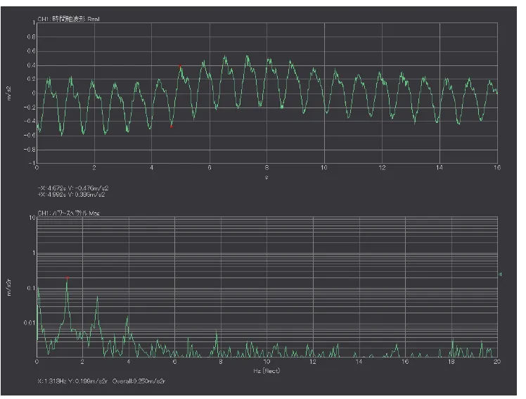
Fig.1 Acceleration time waveform of pendulum (upper), Power spectrum (lower)
Velocity and displacement time waveform obtained from time-axis calculus
The DS-0321 FFT analysis function has the time-axis calculus function. The figure 2 shows that the acceleration time waveform of pendulum, velocity time waveform and displacement time waveform obtained from time-axis calculus. Although the time length of FFT frame is 16 seconds, 8 seconds of that is enlarged.
Looking at the cursor values of velocity/displacement time waveform, they are extremely abnormal values: -499 mm/s, -3256 mm. Also, they look like arch-shaped waveforms. This is because the low frequency noise is emphasized by integration. Thus, they are not the correct waveform of velocity/ displacement.
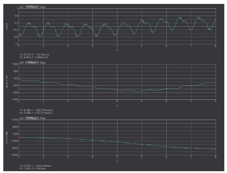
Fig. 2 Acceleration time waveform of pendulum (upper),
integrated velocity time waveform (middle) and integrated displacement time waveform (lower)
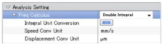
Time-axis differential/integral function is set in the Analysis setting menu 🡪 Time axis data analysis (Figure 3). The velocity time waveform can be obtained by performing a single integration with the time axis differential/integral for the time waveform of acceleration. A displacement time waveform can be obtained by performing double integration. The DC removal is ON. If integration unit conversion is ON, specify the unit of velocity/displacement.
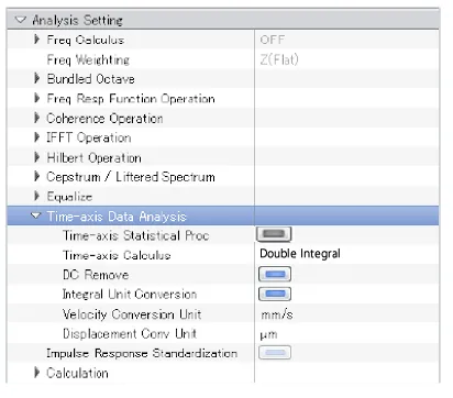
Fig. 3 Display screen of Time-axis calculus function
Velocity time waveform and displacement time waveform obtained from IFFT function
To obtain the velocity time waveform and displacement time waveform from the acceleration time waveform to eliminate the influence of low frequency noise, the frequency calculus function and IFFT (Inverse Fourier transform) function are used.
Perform FFT on the acceleration time waveform once, and obtain the Fourier spectrum.
Divide each frequency component of the Fourier spectrum by (2 × π × frequency) once or twice, and then the Fourier spectrum of velocity and displacement can be obtained.
Figure 4 shows the IFFT (Inverse Fourier Transform) of the Fourier spectrum of velocity and displacement after cutting the components below 1 Hz.
The peak-peak values of the velocity time waveform and the displacement time waveform are 81.8 mm/s and 10.1 mm, respectively, which are appropriate values.
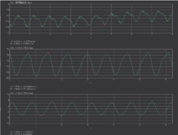
Fig. 4 Acceleration time waveform of pendulum (upper),
velocity time waveform by IFFT (middle) and displacement time waveform by IFFT (lower)
The procedure for displaying the velocity/ displacement time waveform by IFFT function is as follows.
(1) Input/output setting menu 🡪 Window function setting 🡪 Set “Rectangular”
(2) Data display setting 🡪 Data setting 🡪 Fourier spectrum is displayed on the active graph screen.
(3) Analysis Setting 🡪 Frequency calculus 🡪 Select “Single or Double” integral. The integral unit conversion is on, and set speed/ displacement conversion unit.
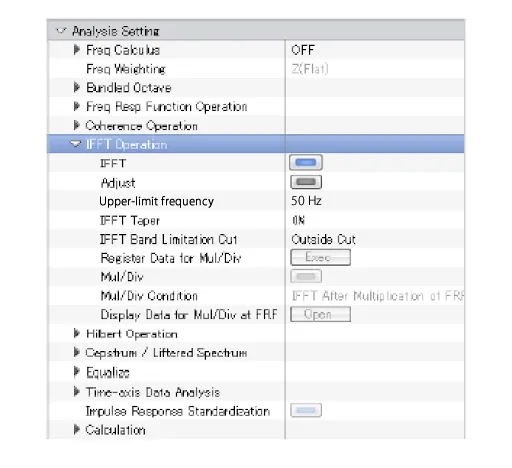
(4) Analysis setting 🡪 IFFT operation, turn on the Band limitation, set the band limitation cut to“Cut outside”, and then turn on the IFFT function. Set the lower-limit frequency to the value that is not affected by low frequency noise. If the time waveform does not become the expected waveform, adjust the lower-limit frequency.
Set the upper-limit frequency to the same value as the frequency range.
Summary
This time, I explained the procedure to convert the time waveform of acceleration into the time waveform of velocity / displacement using the IFFT (Inverse Fourier Transform) function. If the velocity/ displacement time waveform obtained by numerical integration of the time waveform does not become the expected waveform, use the IFFT function.
(Y·K)