No.38 The procedure of FFT time trend analysis in DS-3000 series

In this column, we explain how to display the power spectrum as the time trend. DS-0322 tracking analysis function is required.

Display screen of DS-0320 and Record File Viewer

Displaying DS-0320 as in Figure 1 and Record File Viewer as in Figure 2.

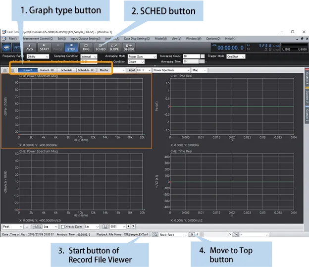
Fig.1 Screen of Sound and Vibration Real-time Analysis software DS-0320

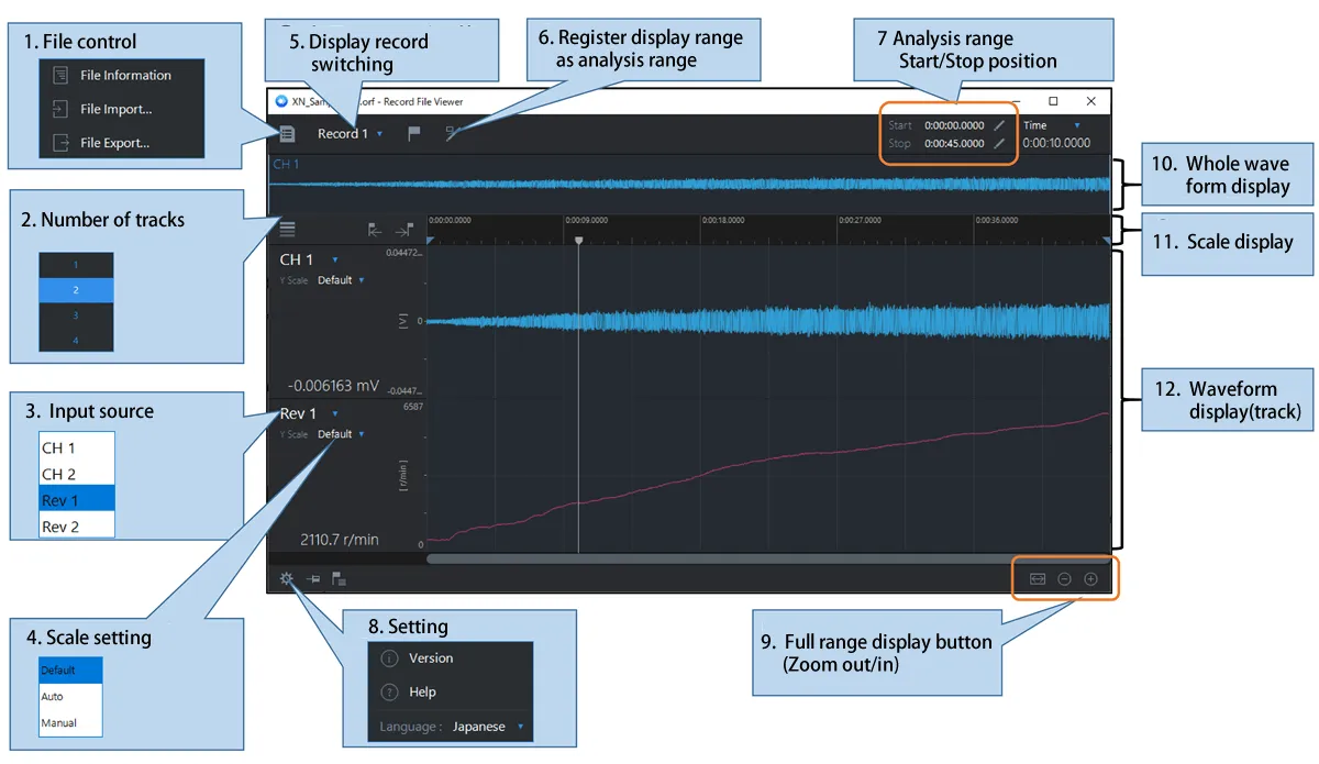
Fig. 2 Screen of Record File Viewer

The procedure to open the record file and perform FFT offline analysis

Open the record data from DS-0320 File menu ”Open Offline Analysis Data” (Figure 3). Select the mode as “FFT (Offline).

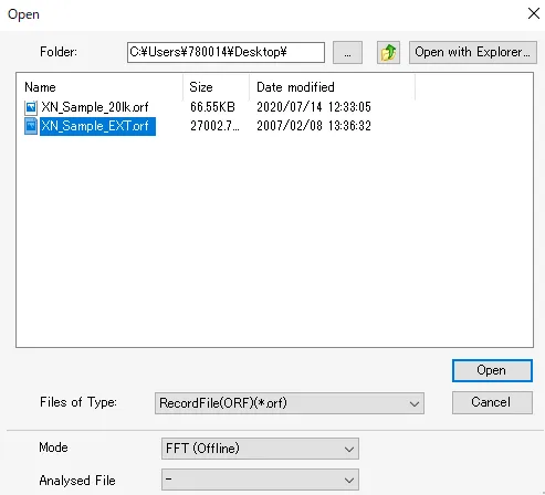
Fig.3 File menu Open Offline Analysis Data dialog

If the record data contains multiple recording results (records), start the Record File Viewer (Figure 1- 3) and select the target analysis record by the display record switching (Figure 2-5 ). If you want to analyze only a certain time range instead of the entire record data, specify the analysis range using “Register display range as analysis range" (Figure 2-6) or "Analysis range" (Figure 2- 7).

If you press the Move to Top button on the DS-0320 (Figure 1- 4) and then press the START button, the entire record data or the specified analysis range will be analyzed sequentially from the beginning, and the analysis will stop at the end position of the range.

How to perform the time trend analysis of the power spectrum

The tracking analysis function (schedule analysis function) is used for the time trend analysis.

Input/output setting → Schedule setting to open a dialog. (Figure 4) Turn off the “SCHED” button (Fig.1-2) before operation. Select “Regular Time Schedule” in Schedule Mode. Set “Interval” and “Total Completion Time” in Regular Time Schedule. If the interval is set to 0.1 seconds and the total time is set to 50 seconds, a total of 500 FFT calculations are performed once every 0.1 seconds to obtain a power spectrum for 500 times. The upper range of the number of calculations is 1000, thus set the interval and total time within the range that does not exceed this range.

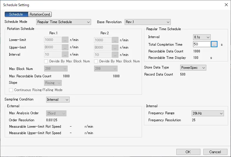
Figure 4. Input/output setting → Schedule setting dialog

Select “Schedule with the graph type button (Fig.1-1). Specify the analysis range you want to analyze with the Record file Viewer, turn on the “SCHED” button (Fig1-2), press the “Move to Top” button (Fig.1-4), and then press the START button to perform schedule analysis. Data display setting  Trance line setting to open the dialog of the trace line setting (Fig.5). By turning Line 1 to Line 8 ON, you can display a graph showing how the frequency component specified by the trace frequency changes during the total time. By turning on “Overall”, the time variation of overall (the sum of all frequency components) can be displayed. P.Overall is the sum of the components in the specified frequency range.

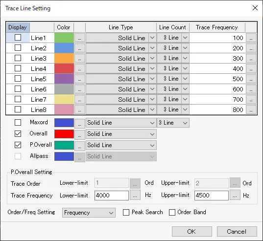
Figure 5. Data display setting → Trace line setting dialog

The result of time trend analysis of the power spectrum is shown in Figure 6.

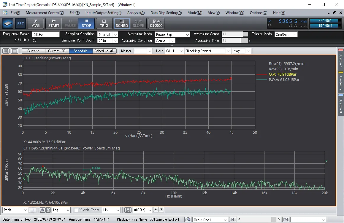
Figure 6. Time trend analysis of the power spectrum

The setting of the Fig.6 as follow: Frequency range: 20 kHz, Sampling points: 2048, Frequency resolution: 25 Hz. The length of the time waveform is 40 ms, which is reciprocal of the frequency resolution. The interval of Regular Time Schedule is 0.1 second (100 ms). Thus, the analysis data will be missed since 60 ms (=100-40) is not analyzed. If you want to calculate all time data, reduce the frequency resolution or shorten the interval of Regular Time Schedule to perform analysis.

Summary

In this column, we have introduced the procedure for time trend analysis of the power spectrum in DS-3000 series. As for the offline analysis, refer to Q & A about measurement, No. 33 & 35,

 

 

(YK)