No.22 Why does the power spectrum scale change depending on measurement conditions or FFT analysis condition?
When looking at power spectrum by analyzing the time waveform of sound and vibration by FFT analysis, the numerical value is much smaller than you expect and you’re puzzled that the numerical value is changed by changing the number of sample points or the frequency range, although the operating condition of the rotating machinery is not changed. Even the vibration and sound is steady, the numerical values may change if the frequency range or analysis conditions are changed.
We explain about the causes related to the signal time waveform and measurement / analysis conditions (FFT analysis habits).
Please refer to the following columns.
https://www.onosokki.co.jp/HP-WK/eMM_back/emm80.pdf
https://www.onosokki.co.jp/HP-WK/eMM_back/emm81.pdf
Waveform with changing frequency (Example: when the rotation speed of machinery is getting fast)
Since the rotation speed is changing, the frequency synchronized with the rotation is also changing.
For a sine wave with a constant frequency of 100.0 Hz as shown in Fig. 1, the power spectrum has a value only at that frequency.
The time waveform in Fig. 1 has an efficient value of 10. 0 m/s2 as the half amplitude is 14 m/s2.
Both 100.0 Hz and overall value is 10. 0 m/s2.
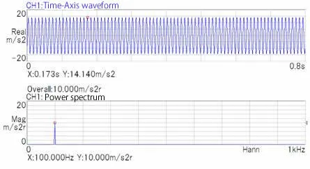
Fig.1
How about the time waveform in Fig.2?
The amplitude is constant but the frequency is changing from low to high.
The time waveform in Fig. 2 has an efficient value of 10. 0 m/s2 as the half amplitude is 14 m/s2.
The frequency is changing between 130 Hz and 480 Hz for 0.8 second.
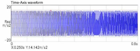
Fig. 2
Since the half amplitude value is 14.14 m/s2, the power spectrum of each frequency component is expected to be 10.0 m/s2, but this does not apply to FFT analysis. The power spectrum is equivalent to the mean square value of each frequency component included in the time waveform.
Since the frequency is changing, the existing ratio of each frequency components is low in 0.8 second. The magnitude is 0 when there is no frequency component. The average result for 0.8 second becomes smaller depending on the existing ratio.
The overall value is 10.0 m/s2. (performing FFT by 1 kHz, 2048 points)
In figure 3, the second screen from the top is FFT analyzed with a Hanning window and the third one is FFT analyzed with rectangular window.
The effect of time change and the shape of the time window are clearly shown in the power spectrum distribution.
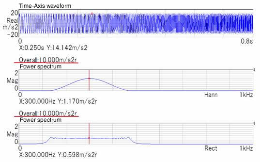
Fig.3
Waveform with weighting Hanning window
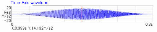
Fig.4
The maximum weighing of Hanning window is the middle of time (0.4s) (Fig. 4)
The frequency component is large at that point.
As for the rectangular window, the frequency component is distributed evenly as the weighing is consistently 1. (It is affected by the way of cutting out waveform.)
The magnitude at 300 Hz is 1.17 m/s2 in Hanning window, 0.598 m/s2 in rectangular window.
The Hanning window compensates for the decrease caused by the window functionality, so a larger value was obtained than the rectangular window, but it was far from 10.0 m/s2.
The half amplitude of the time waveform is 14.14 m/s2, the result of the power spectrum is smaller. It means that each frequency component exists for a short time for 0.8 second.
The magnitude obtained in the power spectrum is equivalent to the root mean square value of the time waveform for each frequency component. If it is the same frequency for 0.8 second, it will not decrease when averaged, but if the frequency is changing and the existence time for 0.8 second is short, it will decrease by the proportion of existence when averaged.
There are the measurement conditions which FFT time length and the ratio of existence time of frequency component are changing; one is setting the number of sample points, another is setting the frequency range.
How about the number of sample points increase from 2048 to 4096?
The efficient value is 10. 0 m/s2 as the half amplitude is 14 m/s2 constantly. The change in frequency increases as time increases from 0.8 second to 1.6 second. The time ratio of a certain frequency component to the time length is reduced to 1/2. Since the value of the frequency component is the mean square value within the time length, it decreases as the ratio decreases. The overall remains unchanged as 10.0 m/s2.
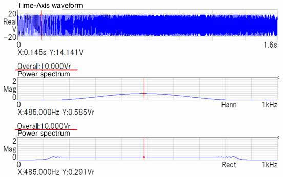
Fig.5
The efficient value is half compared to 2048 points.
It is same when the frequency range is reduced. When the frequency range is reduced, the time length is longer.
The phenomenon that the value changes depending on the measurement and analysis conditions also occurs in random waveform.
The differences in value due to the time length also appear in the case of the waveform (random signal) in which the power spectrum is continuously distributed. The random waveform is changed according to the frequency resolution (⊿f).
Even though the signal is the same, the number of sample points is different. Or even though the number of sample points is the same, the frequency range is different. The values are changed in these cases.
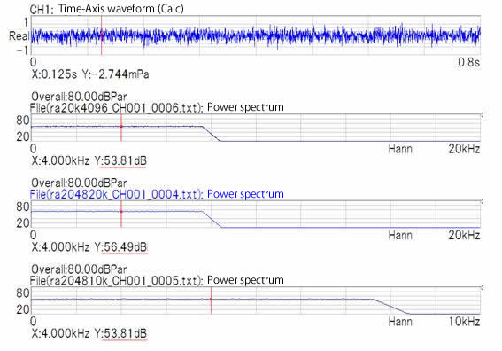
Fig6
The time length varies depending on the number of sample points and the frequency range. As a result, the value changes accordingly. When measuring, it is necessary to keep a record of the operating conditions of the equipment, the measurement and analysis conditions.
(H.K)